There are many instances when one wants to show two different measurement scales each of which measures the same data. One such instance would be showing temperature readings in both the Fahrenheit and the Celsius scales as in Figure 1, which shows the mean soil temperature through the summer months using both temperature measurement systems. For technical reasons discussed below, the best that is possible is to simulate the effect. We will plot two series but make it look as though the chart contains just one.
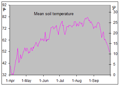
Figure 1
What we need to know, obviously, is how the two systems
relate to each other. In the case of temperatures, the relationship is ![]() ,
where C is the temperature in Celsius and F is the temperature in
Fahrenheit.
,
where C is the temperature in Celsius and F is the temperature in
Fahrenheit.
There are two key elements to remember in simulating the effect of a single chart with two axes. First, Excel will create a secondary axis only if we plot at least 2 series in the chart. Second, since the two measurement scales are different we will have to calculate the temperatures in each of the two systems.
Consequently, we will plot the data as recorded in Fahrenheit and as calculated in Celsius, move the Celsius series to the secondary y-axis and align the two axis (minimum and maximum scale values) so that the two series overlap so precisely that it appears as if the chart contains just the one series. The key to getting the two series to overlap is aligning both the minimum and the maximum values on the two axes. Of course, aligning does not mean having the same values but having values that represent the same temperature. For example, if we wanted the minimum and maximum values to be the freezing and boiling temperatures of water, respectively, we would have 32 and 212 as the minimum and the maximum values on the primary axis with the corresponding values on the secondary axis being 0 and 100.
|
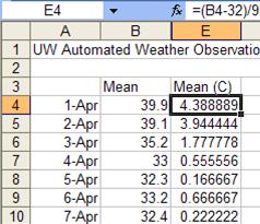
Suppose the actual data (observation date and temperature in °F) are in columns A and B. Then, calculate the readings in °C using the formula in the Concepts section. The result is as shown in Figure 2. |
Figure 2 |
|
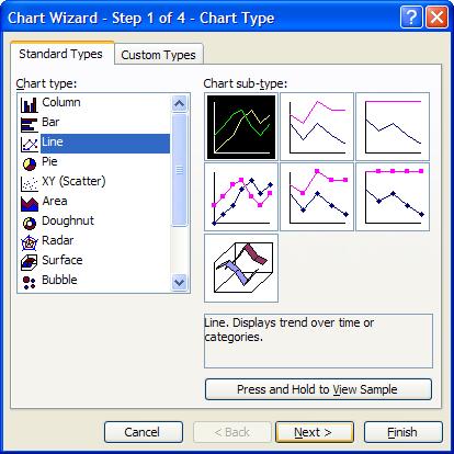
Now, use the data in columns A, B, and E to plot a line chart as in Figure 3. The result is shown in Figure 4. |
Figure 3 |
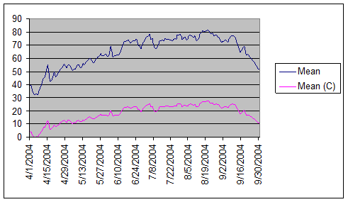
Figure 4
Delete the legend (select the legend and press the Delete key). Hide the y-axis gridlines (select the chart, then Chart | Chart Options… | Gridlines tab | in the Value (Y) Axis section uncheck the Major Gridlines checkbox.
|
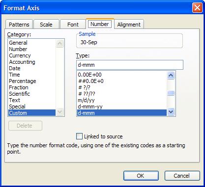
Change the format of the x-axis to a date format of d-mmm. Before closing the dialog box… |
Figure 5 |
|
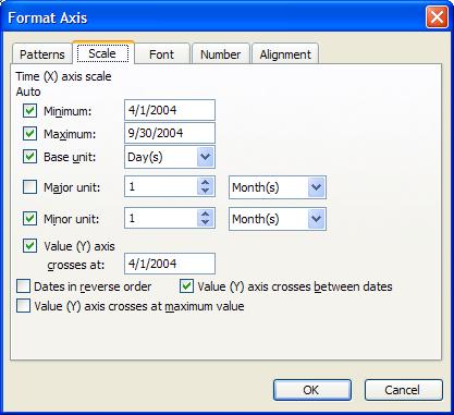
…set the scale to a major unit of 1 month. |
Figure 6 |
Move the series corresponding to Mean (C) to the secondary axis (double-click the plotted series then select the Axis tab, then select the Plot series on Secondary axis option). Ensure that the pattern remains a line with no markers.
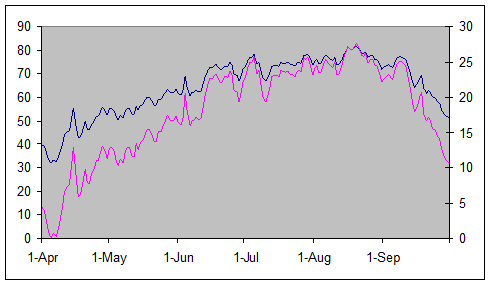
Figure 7
Note that the shapes of the two series are starting to look alike. The chart has the values in Fahrenheit on the primary y-axis and in Celsius on the secondary y-axis. Clearly, the minimum temperature, which happens to be in the first few days of April, is a little above freezing, which is 32°F or 0°C. So, we will rescale the primary y axis to have a minimum value of 32°F as in Figure 8 while ensuring that the secondary y-axis minimum value remains 0°C.
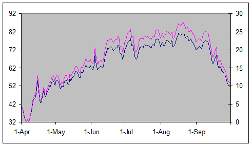
Figure 8
The result is that the two series are starting to overlap.
Excel has set the maximum value for the primary y-axis as 92°F. This
corresponds to ![]() or a Celsius
value of 33.33°C. Hence, we should have a maximum value of 33.33 on the
secondary y-axis (while ensuring the minimum remains 0). As soon as we do
that, the two series overlap precisely (Figure 1).
or a Celsius
value of 33.33°C. Hence, we should have a maximum value of 33.33 on the
secondary y-axis (while ensuring the minimum remains 0). As soon as we do
that, the two series overlap precisely (Figure 1).