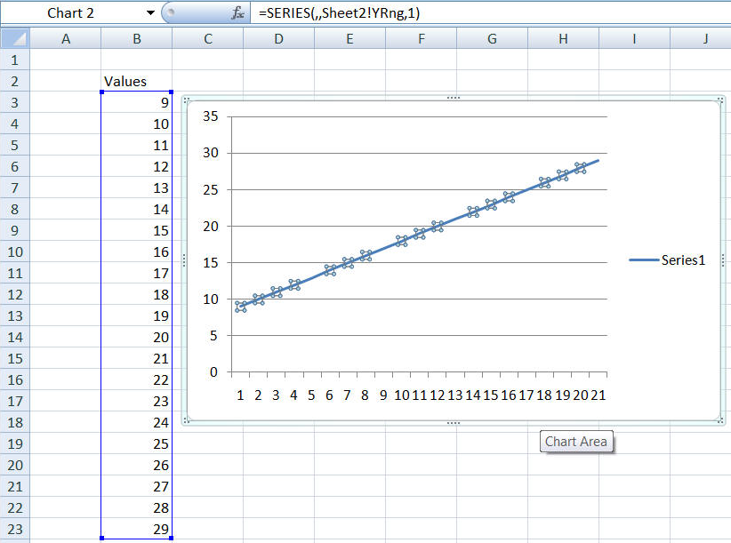
On this page I discuss more advanced applications of the basic technique demonstrated on the Dynamic Charts page.
In the basic setup, the OFFSET function relies on an 'anchor cell' - the first argument to the function. But, consider the scenario where one plans to add new data at the bottom of the data range and subsequently delete the older data towards the top.
The 'simple' dynamic range formula that we have used so far looks like
SimpleDynamicRng =OFFSET(Sheet2!$B$3,0,0,COUNTA(Sheet2!$B:$B)-1,1)
Now if one were to delete row 3 the named formula would contain an error
SimpleDynamicRng =OFFSET(Sheet2!#REF!,0,0,COUNTA(Sheet2!$B:$B)-1,1)
The way around this is to use the INDIRECT function to refer to cell B3. This fairly straightforward approach uses the named formula
IndirectDynamicRng =OFFSET(INDIRECT("B3"),0,0,COUNTA(Sheet2!$B:$B)-1,1)
However, it will not work because the Excel charting module requires one to qualify the range reference with the worksheet name. If on were to use the IndirectDynamicRng name in a chart, Excel would show the below error message.

One way to fix this issue is to include the name of the sheet in the INDIRECT function. But that leaves the solution vulnerable to the sheet name being changed - something analogous to the deletion of the anchor cell. So, we need to find the name of the worksheet dynamically, and then use this name in the range formula.
For any saved workbook the CELL function with the first argument of "filename" returns the entire file name including the worksheet name. One then has to extract the worksheet name from the returned result. The named formula SheetName does just that. Then, the dynamic range formula uses this SheetName in computing the range of interest.
SheetName	="'"&MID(CELL("filename",INDIRECT("b1")),FIND("]",CELL("filename",INDIRECT("b1")))+1,255)&"'"
YRng 		=OFFSET(INDIRECT(Sheet2!SheetName&"!b3"),0,0,COUNTA(Sheet2!$B:$B)-1,1)
