You are on the Home/Excel/Tutorials/Worksheet as Gantt Chart page

Using a Worksheet for a Gantt Chart - I

One application of an overlooked capability is the ability to format Excel worksheet cells so that the final result is that they convey information visually rather than through numbers.  There are many applications of this technique such as creating a Gantt chart.

A Gantt Chart

The layout for the data is as shown below.  Task specific information is in columns A and B with the the start and end dates in columns C and D respectively.  Row 1 starting with column E has calendar dates.

What we want is to see the grid encompassed by the columns on the left and the row at the top filled with the appropriate color for those dates when a particular task is scheduled.

The above is quite easy to do.  Select E2 and set its conditional format as below.

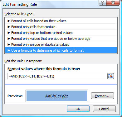
with the format set to the desired color.

Now, copy E2 to the entire range that represents the grid identified by the columns on the left and row at the top.  This will create the desired visual effect of a Gantt chart.