Excel's PivotTable includes a built-in 'Top 10' capability where the 10 is a customizable number. However, there is no way to get a consolidated summary of the rest of the categories, essentially, no way to see something like:
This tip illustrates two ways to get the desired result. The first approach is easy to implement but it does not scale if the Top 10 list changes in length as might happen if one were to customize the 10 or if there are multiple categories in the last place in the list all with the same value in which case there will be more than 10 items in the list. In the example below, the PivotTable shows a Top 3 list. However, because what would be in the 3rd place has two categories, each with a value of 5, the list consists of 4 items.
The 2nd approach uses a set of formulas that dynamically adjust to a varying length for the Top 10 list.
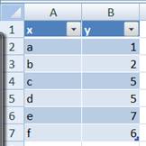
Suppose the original data are as shown below with the first row containing the column labels.
From this create a PivotTable where the column labeled 'x' is the Row Field and the column labeled 'y' is the data field. By default Excel puts the PivotTable on a new worksheet and creates a Sum statistic, both of which are just fine for this analysis.
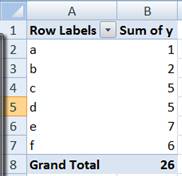
Figure 1
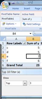
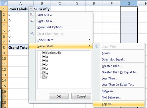
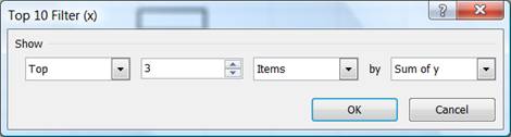
With the PivotTable in place, select the Row Labels drop down then the Value Filters submenu and finally the Top 10... filter as shown below. In the dialog box, change the default Top 10 to Top 3.
Now, the PivotTable will look like below.

Figure 2
The PT displays 4 rows even though the filter indicates a Top 3 request. This is because two categories (c and d) both have the 3rd highest value (5).
With the basic PivotTable constructed, we can start on the actual task at hand. For starters we need to know the total of all the elements not shown in the above PT. This is relatively easy since it is the difference between the sum of all the elements less the Grand Total shown above. To get the total for all the elements, create a 2nd PivotTable that has the y column as the data field but no row field or column field.

Figure 3
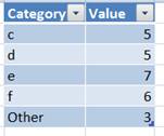
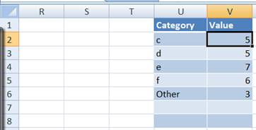
Next, in some empty range, say L2 enter the formula =A2 (this is the first cell with data in the first PT). Copy L2 to M2 and copy L2:M2 down to 3:5. This essentially duplicates the PT values outside the PT. Format the cells as desired.
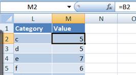
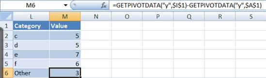
In L6 enter the word 'Other' and in M2 enter the formula shown below. The easiest way to do this is to enter the = key, then click the mouse in the cell containing the data in the 2nd PT (I2 in the example above), the - key, and finally click the mouse in the cell with the Grand Total in the 1st PT (B6 in the above example).
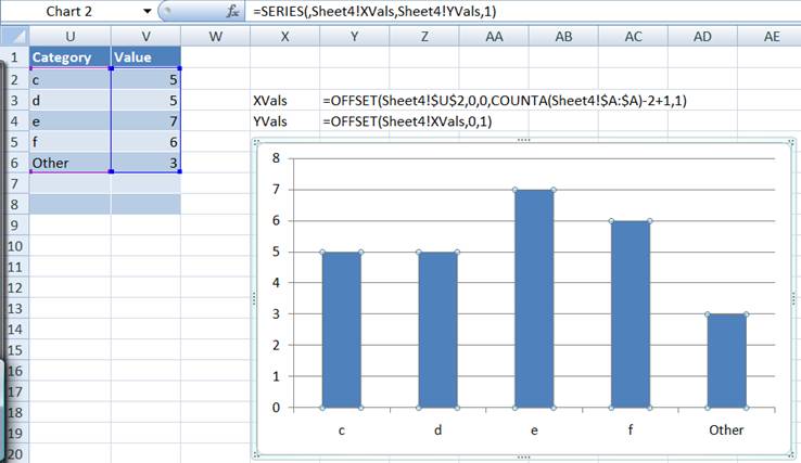
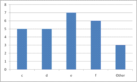
Select L2:M6 and create a Column chart to finish the job and we are done!
The obvious problem with this approach is that if the Top 3 is changed to Top 5 or if in the original data set the value for d changes from 5 to 4, the above approach will require us to redo our work.
We will use the same data as above (Figure 1) and the 2 PivotTables (Figure 2 and Figure 3). In some cell, say U2 enter the array formula shown below. To enter an array formula, complete formula entry with the CTRL+SHIFT+ENTER key combination rather than just the ENTER (or TAB) key. If done correctly, Excel will show the formula within curly brackets { and }.
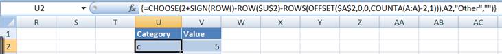
The formula above shows the category from the original PT if the row is less than or equal to the number of rows of data in the PT. If it is one more, it shows the literal 'Other' and the zero length string "" for all other values. In V2 enter the formula
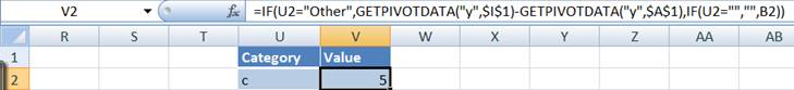
Copy U2:V2 down the columns until there is at least one cell with a zero length string. Format the range as desired.
Finally, to create a dynamic chart, use the usual technique. Create two names as shown below and use them in the chart.