There are many instances where the data set is a table laid out as in Figure 1. The first row and the first column describe the contents of each column and row respectively.
Figure 1
1) The first requirement is to find the entry at the intersection of a particular value of the first column and the first row. For example, look up the value for Product KK and Category F.
Figure 2
2) The second requirement is to find, given the value for a product, the category with the minimum value. The example below (Figure 3) looks up the minimum value for Product JJ and then finds the corresponding category, G.
Figure 3
There are variants of this requirement that have the same solution adjusted as required. It could be to find the product that yields the minimum value for a particular category, i.e., go in the opposite direction of the above arrows.
Of course, instead of looking for the minimum, one might also want to look up the maximum.
The idea here is to use INDEX to locate the row and column of interest within the data area. To identify the row and column of interest, use the MATCH function.
So, suppose the above table is in Sheet1 and in Sheet2 we have a set of products to look up for a particular category:
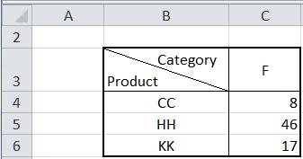
Figure 4
In cell C4 enter the formula =INDEX(Sheet1!$C$3:$I$13,MATCH($B4,Sheet1!$B$3:$B$13,0),MATCH(C$3,Sheet1!$C$2:$I$2,0))
Copy C4 down to C5:C6.
This is slightly more complex but not much more. Use the INDEX and MATCH functions in a different sequence to get the desired result.
Figure 5
Suppose we have several products in Sheet2!E4:E6 (see Figure 6). The solution is intentionally broken up into discrete steps.
F4 contains the formula =MATCH(Sheet2!E4,Sheet1!$B$3:$B$13,0), which identifies the row within the data that contains the product in E4. The result of 3 means it is in the third row of the data.
G4 contains the formula =MIN(INDEX(Sheet1!$C$3:$I$13,Sheet2!F4,0)). The zero as the second argument of the INDEX function tells Excel to use the entire row identified by the first argument.
Finally, H4 contains the formula =INDEX(Sheet1!$C$2:$I$2,MATCH(Sheet2!G4,INDEX(Sheet1!$C$3:$I$13,Sheet2!F4,0),0)). The innermost INDEX isolates the row of interest. The MATCH identifies the column containing the minimum value, and the outer INDEX locates the category of interest.
To do the same for the other products of interest in E5:E6 copy the formulas in F4:H4 down to rows 5:6.
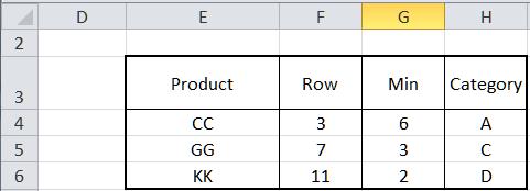
Figure 6