Ordinal numbers convey information about the order of elements in a set. They show rank or position but there is no information about quantity. “First” and “second” are both ordinal numbers but they do not say anything about the distance between first and second. If “first” and “second” were the ranks of two students in a class, there’s no way to know whether the two students were separated by a fraction of a point (the person ranked first might have scored 95.4 and the person ranked second might have scored 95.3) or they might be far apart (for example, 95 and 75, respectively).
The number associated with the rank is usually followed by a suffix as in 1st, 2nd, 3rd, 4th, etc. The rules for adding these suffixes are as follows:
1) If the number ends in the digits 11 through 20, add ‘th.’ The way to find if a number ends in 11 through 20 is to check number modulo 100 (i.e., the remainder from dividing the number by 100).
2) If rule 1 does not apply, then check the ending digit (use number modulo 10 to get the last digit). If it is 1, add ‘st.’ If it is 2, add ‘nd.’ If it is 3, add ‘rd.’
3) If neither rule 1 nor rule 2 applies, then add the suffix ‘th.’
Starting with Excel 2007, it is possible to specify the number format as part of conditional formatting. This note shows how to leverage that capability to add the appropriate suffix to an ordinal number.
The default number format will be 0”th”. This takes care of rule 3 above, i.e., if neither rule 1 nor rule 2 apply to the number, it will have the suffix “th.”
Select the cell (or cells) containing the ordinal numbers. In the example I used, I had numbers as shown below.
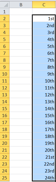
Figure 1
Then, select Home tab | Styles group | Conditional Formatting dropdown | New Rule… button.
In the Edit Formatting Rule dialog box, select Use a formula to determine which cells to format and enter the formula =AND(MOD(C2,100)>10,MOD(C2,100)<21). Then, click the Format… button to specify the conditional format.
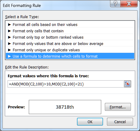
Figure 2
In the resulting Format Cells dialog box, select the Custom category, and enter the custom format 0"th".
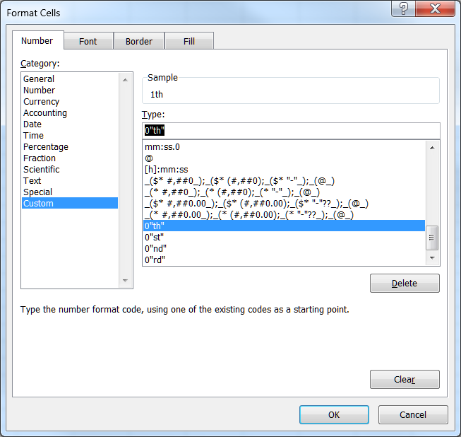
Figure 3
Close all open dialog boxes by clicking the respective OK buttons.
Actually, there are three conditional formats, one for each of the “st,” “nd,” and “rd” suffixes.
For each, start by clicking the Home tab | Styles group | Conditional Formatting dropdown | New Rule… button.
In the Edit Formatting Rule dialog box, select Use a formula to determine which cells to format.
Then, enter the formulas and the corresponding conditional number formats shown below.
=MOD(C2,10)=1 Custom format: 0"st"
=MOD(C2,10)=2 Custom format: 0"nd"
=MOD(C2,10)=3 Custom format: 0"rd"
Make sure that if rule 1 applies to a cell, Excel does not subsequently apply rule 2. To do that, in the Conditional Formatting Rules Manager dialog box check the box each of the checkboxes Stop If True.
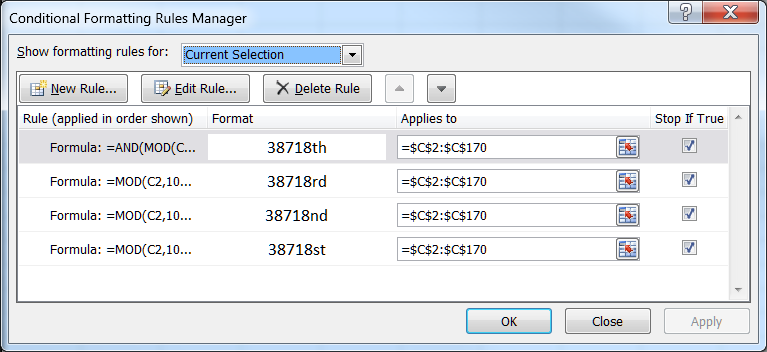
Figure 4