When working with a worksheet that contains a large number of rows and/or a large number of columns with row and column headers, it is very helpful to always view the headers no matter where one scrolls through the document.
An example is in Figure 1. The table lists the year-by-year carbon dioxide emissions by country (the data set comes from data download page at Gapminder – http://www.gapminder.org/data/). The current worksheet view shows data from the 1950s (columns GQ through GZ) and countries that are alphabetically towards the end of the list of countries (rows 235 through 259). At the same time, the column headers (row 1) and the row headers (column A) are still visible. This lets one quickly establish a context for the numbers. Figure 1 is the result of using Excel’s Freeze Panes feature.
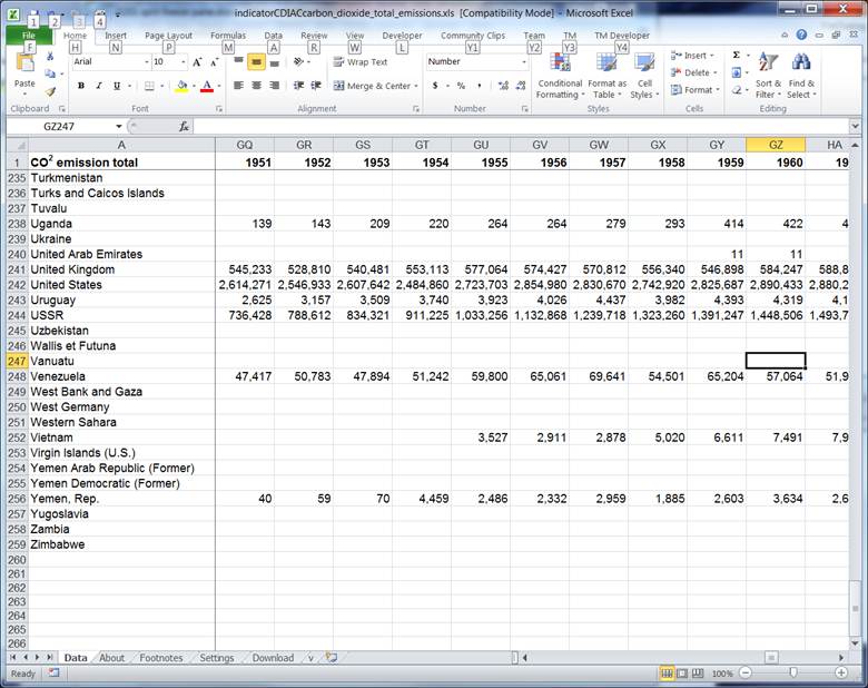
Figure 1 – Freeze Panes set at row 1 and column A show that row and column no matter where one scrolls in the worksheet
A complementary feature is called Split Panes (see Figure 2). The key differences between freeze pane and split pane are the somewhat different behavior while scrolling and an easier way to adjust the panes, which, of course, comes with extra responsibility to manage the risk of accidental changes to the split panes configuration.
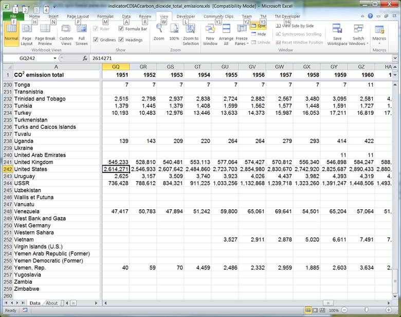
Figure 2 – Split panes set ar row 1 and column A look similar to freeze panes but each pane supports scrolling through the entire worksheet and the splits are easy to adjust by dragging the gray split bars
Select the cell that will be the top-left cell of the main pane in that the split freeze will occur to the left of the selected cell and above the selected cell. So, in the example shown in Figure 3, select cell B2. Then, select View tab | Window group | Freeze Panes dropdown > Freeze Panes button.
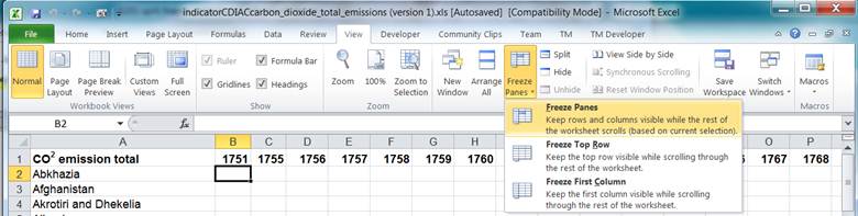
Figure 3
To create only a vertical freeze (i.e, have two panes one on top and the other below), select the entire row that will be the first row in the bottom pane and then select the Freeze Panes button as above.
Similarly, to create only a horizontal freeze with two left and right panes, select the column that will be the first column in the right pane and then select the Freeze Panes button as above.
Other options are Freeze Top Row and Freeze First Column. These two options work independent of the current selection in that they will freeze just the first row or the first column, respectively.
To remove the frozen panes, select View tab | Window group | Freeze Panes dropdown > Unfreeze Panes button.
As noted earlier, once Freeze Panes is active, scrolling will not affect the frozen rows and/or columns. In Figure 1, scrolling right to columns GQ:GZ still shows the country names at the left in column A and scrolling down to rows 235:259 still shows the years at the top in row 1.
One can think of each pane as spanning a portion of the worksheet. In our example, the top-left pane spans only 1 cell (A1). The top right pane spans row 1 of all the columns from B to the right. The left bottom pane spans only column A of all the rows from 2 on down. Finally, the large bottom-right pane spans B2 to the last cell in the worksheet.
Consequently, if one selects a cell at the pane boundary, say cell B2 and then uses the arrow key to move left (or up), Excel will simply select the cell in the frozen pane. So, after selecting B2, if one were to use the left-arrow key to move left, the result is that cursor moves to the frozen pane and selects cell A2.
This is similar to Freeze Panes with some differences in behavior and flexibility. There are two ways to activate Split Panes. The first is similar to the Freeze Panes process. Select the cell that will be the top-left cell of the main pane in that the split freeze will occur to the left of the selected cell and above the selected cell. Then click View tab | Window group | Split button.
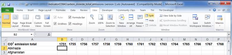
Figure 4
The result (see Figure 5) looks similar but somewhat different from Freeze Panes. The demarcation between the panes is a thicker grey bar rather than the earlier thin black line.
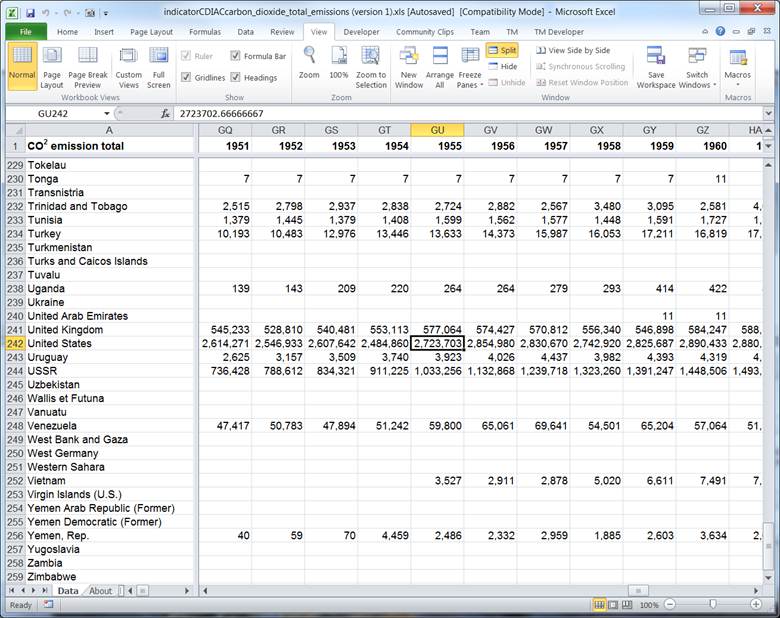
Figure 5
Just as with Freeze Panes, select an entire row or an entire column to create only a vertical split or a horizontal split. Figure 6 shows how to create two vertical split panes
Figure 6 – Create 2 vertical panes (top and bottom) by selecting an entire row and then clicking the Split button. Achieve a similar result for horizontal (left and right) panes by selecting a column before clicking the Split button.
The other way to create a split pane is to use one of the pane split boxes. These are relatively inconspicuous controls at the top of the vertical scroll bar and at the right of the horizontal scroll bar. Click and drag the control to the location of the desired split (Figure 7).
Figure 7 – An alternative way to create split panes.
For the most part ‘split panes’ provides functionality similar to ‘freeze panes.’ The two important differences are the following:
1) The splits are easy to adjust. Simply move the mouse over one of the grey split bars and click-and-drag to a new location. The vertical bar, which creates the left and right horizontal panes, moves left or right. Similarly, the horizontal bar, which creates the top and lower vertical panes, moves up or down.
Dragging the bar to the extreme right (or the extreme top) will remove the split pane.
2) Each of the split panes actually spans the entire worksheet. This is very different from the freeze panes behavior, where each pane spans only a portion of the worksheet. With the cursor in any pane, say the bottom-right main pane, scroll all the way up or all the way left and Excel will show the contents of the top (or left) pane in the active pane! For example Figure 8 shows the result of scrolling the main pane all the way to A1. While the header panes show their own content, the main pane duplicates that content.
Clearly, this is something that can get confusing, especially if one selects a cell in one of the header panes and then scrolls, something that has been known to happen, usually by accident.
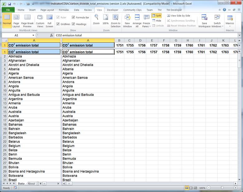
Figure 8 – Each split pane spans the entire worksheet. Consequently, it is possible to select A1 in the main pane. While this capability is useful at times, the result may confuse the unsuspecting consumer. The view may be even more confusing after scrolling in one of the header panes.
Excel 2010, Excel 2007, freeze panes, split panes, view, scroll worksheet