A couple of days ago, I overheard my fiancée helping her nephew as he struggled with Conway’s Game of Life in his introductory course on computer programming. I hadn’t thought of this simulation in a long, long time and decided to see if I could do it in Excel.
For an introduction to the simulation see http://en.wikipedia.org/wiki/Conway%27s_Game_of_Life.
The first attempt was primarily in VBA with Excel used simply to show the result. It turned out to be an interesting exercise since I decided to make it a test case for an add-in meant to work in Excel 2003 through Excel 2010 both 32-bit and 64-bit and on Mac Excel 2011. I’ll probably share that experience at a later date.
Then, I decided to see if I could run the simulation strictly in Excel. No VBA code allowed. This post shares that experience.
A synopsis of the rules for the simulation:
We simulate a ‘universe’ that consists of a grid of cells. Each cell is in one of two states, ON or OFF (also called alive or dead). Each cell has eight neighbors: on the left, on the right, above and below, and the four cells to the top-left, top-right, bottom-left, and bottom-right. The simulation starts with a pre-determined seed state. At each step, the simulation determines a new state of the universe. This happens by determining what happens to each individual cell. There are two simple rules that determine how each cell evolves:
A cell that is currently OFF (dead) becomes ON (alive) in the next iteration if it has exactly 3 live neighbors, i.e., neighbors that are ON.
A cell that is currently ON (alive) remains ON (alive) if it has 2 or 3 ON (live) neighbors. Too few or too many and it turns OFF (dies).
These two simple rules can yield some fairly interesting universes including self-repeating patterns like the two below.

Figure 1 – Blinker
(http://en.wikipedia.org/wiki/File:Game_of_life_blinker.gif)
Figure 2 – Gosper’s Glider Gun
(http://upload.wikimedia.org/wikipedia/commons/e/e5/Gospers_glider_gun.gif)
An important item to note is that the state of the next generation depends strictly on the state of the current generation. What that means is that we use the current state of all the neighbors of a cell and we do not mix-and-match the new state of those neighbors that we might have already calculated with the current state of the other neighbors.
This requirement, then, requires that we have 2 grids, the current grid and the next grid. Once the next grid is fully known, it becomes the current grid and we can then iterate the process.
This post builds the blinker pattern in a 5x5 grid. Starting with a small grid makes it easy to follow the development of the simulation. In addition, scaling the result to larger sizes is very easy and requires no additional conceptual or model changes.
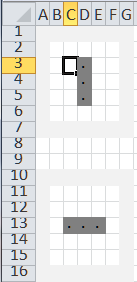
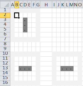
The starting configuration of a particular game is known as the seed. It is similar to the grid used in the evolution but with just starting values. An example of the seed for a blinker pattern is:
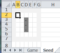
This is a 5x5 grid with a 1 cell border that is shown in light-grey. The “off” cells contain the formula =”” and the ON cells contain a dot (.). Conditional formatting makes those cells appear with a dark fill.
Similarly, the seed for Gosper’s Glide Gun is
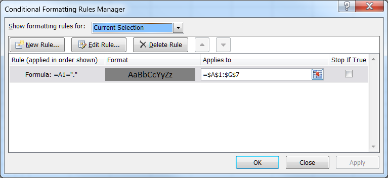
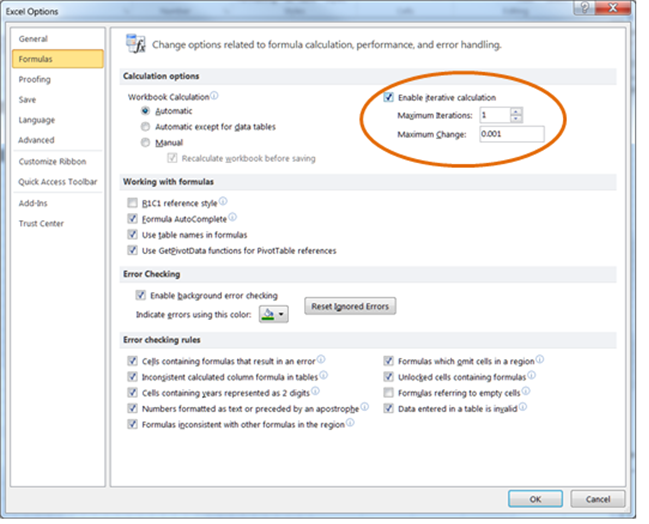
The first thing to note is that since the next state of a cell depends on its current state, we will have to use a recursive formula (known as an iterative formula in Excel). To enable this capability – it is not on by default – select File menu | Excel Options button | Formulas tab | Enable iterative calculation checkbox. Also, make sure that Maximum Iterations is 1.
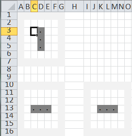
As explained above, the new state of the grid depends on the current state of the grid. The only way to make that happen in Excel is to have two grids, each of which is calculated from the other (this is where the iterative calculation comes in).
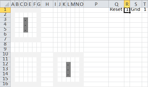
Of course, now that we have 2 grids, we have to designate which one contains the current state. The way to do that is to create a third grid that “points” to the correct grid.
In building an iterative solution – any iterative solution – it is always a good idea to include a ‘reset trigger.’ This forces the iterative solution to reset itself to the starting condition. In addition, in our case, we need a toggle that indicates which is the current state. This toggle will flip between the top grid and the bottom grid.
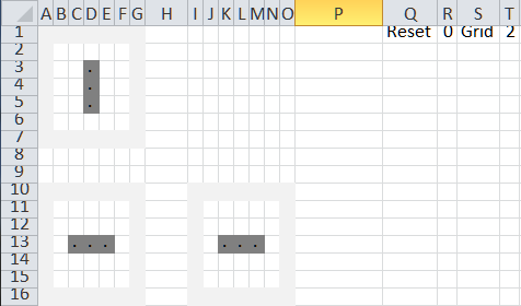
The Reset trigger is a cell in which entering a 1 will lead to a reset. The Grid toggle cell contains the formula =IF(R1=1,1,MOD(T1,2)+1). The formula states that if the game is reset, return a value of 1, which “points” to the top grid. Otherwise the MOD(T1,2)+1 toggles the value between 1 and 2. Note that the formula is in cell T1 and that it refers to the same cell. This makes it an iterative formula.
The 2 rules used in calculating the next state of the game are repeated below:
A cell that is currently dead becomes alive in the next iteration if it has exactly 3 live neighbors.
A cell that is currently alive remains alive if it has 2 or 3 live neighbors. Too few or too many and it dies.
For a cell that is not on the grid boundary it is fairly straightforward to know which cells to use in the calculation. For example, for cell C3 we get the count of the neighboring cells that are on with the formula COUNTIF(B11:D11,".")+COUNTIF(B12,".")+COUNTIF(B13:D13,".")+COUNTIF(D12,".")
But, how about the boundary cells? Do we need specialized formulas for the cells at the four corners, the top and bottom rows, and the left or right columns? At first, it might look like we do. After all, these cells don’t have the 8 neighbors that an inner cell does. But, we can work around this issue by adding an outer ring of cells that will always be off. Now, the boundary cells become inner cells and we can use the same formula for all the cells in the grid!
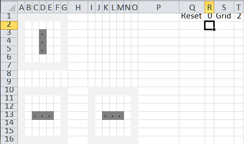
Let’s look at the three that we have. The 2 grids on the left are where the calculations happen. The third grid is the one that shows the current result.
First we address the top grid. Then we look at the lower grid. Finally, we pick which grid is the current grid.
Cell B2 contains the formula
Here’s what the formula does.
The first test, $R$1=1, tests the reset trigger. If it is 1, i.e., the game has been reset, the formula returns the value from the same cell in the seed worksheet.
If the game is active, the next test $T$1=2 checks which of the top or bottom grids contains the current state. If it is 2 then the top grid should remain unchanged. So, the formula returns the current value in the cell itself. This is a recursive, or iterative, result.
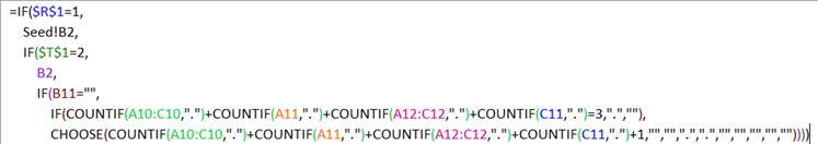
If, on the other hand, we are calculating the top grid ($T$1=1), then the current state is given by the bottom grid. So, the cell references are to the bottom grid. We start by checking if the cell is currently off (B11=””). If that is the case, then in the next generation it will be ON only if exactly three of its neighbors are on. That’s the test IF(COUNTIF(A10:C10,".")+COUNTIF(A11,".")+COUNTIF(A12:C12,".")+COUNTIF(C11,".")=3,".","")
Finally, the cell is currently on and it will remain on only if it has 2 or 3 neighbors that are on. I could have used an OR function.
IF(OR(COUNTIF(A10:C10,".")+COUNTIF(A11,".")+COUNTIF(A12:C12,".")+COUNTIF(C11,".")=2, COUNTIF(A10:C10,".")+COUNTIF(A11,".")+COUNTIF(A12:C12,".")+COUNTIF(C11,".")=3),".","")
Instead, I leveraged the fact that the count of ON neighbors will be a number between 0 and 8. So, I used the CHOOSE function to return either a “” or a “.”.
CHOOSE(COUNTIF(A10:C10,".")+COUNTIF(A11,".")+COUNTIF(A12:C12,".")+COUNTIF(C11,".")+1,"","",".",".","","","","","")
Copy the formula from B2 to all the cells in the grid B2:F6 to complete the calculations for the top grid.
Cell B11 contains the formula
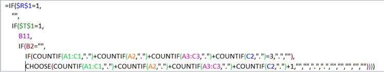
This formula is a “conceptual mirror image” of the formula in B2.
If the game is in reset mode, the bottom grid should be empty. So, the formula returns “”.
If the game is active and the toggle points to the top grid ($T$1=1), the formula returns the value in the cell itself.
If not, then the calculations for the cell being currently ON or OFF are the same as above except now the references are to the top grid rather than the bottom grid.
Copy B11 to B11:F15.
In J11 enter the formula =IF($T$1=1,B2,B11) and copy it to all the cells in J11:N15. This formula selects either the cells from the upper or the lower grid depending on the value of the toggle in T1.
To start the simulation, reset it to the seed configuration. The final grid (J11:N16) shows the upper configuration grid, which is also the seed configuration.
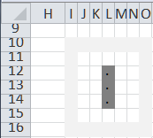
Change the reset trigger to 0. This starts the simulation. The toggle (T1) changes to 2 and the result grid shows the data from the lower grid.
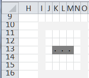
Press F9 (the recalculate keyboard shortcut) and the result grid shows the next generation. Since this is a blinker pattern the two below patterns repeat over and over again.
Here’s one place where VBA might play a role. Write a small macro that repeatedly asks Excel to carry out a recalculation.
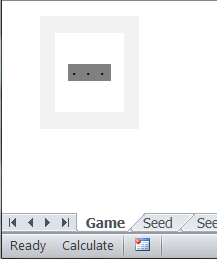
There’s no good reason for the gridlines or the row and column headers to be visible. One can also hide the top and bottom grids, possibly by hiding those columns. The result:
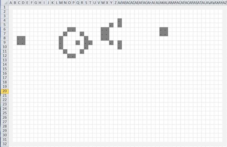
We used the 5x5 grid since it was easy to understand. Luckily for us, the model scales very elegantly. Creating a 30-rows-by-50-columns grid is simply a case of inserting the appropriate number of rows and columns and copying the formulas over to the newly added cells. Below is a snapshot from the Gosper’s Glide Gun simulation.

