One of the most powerful, if not the most powerful, feature of Excel is its array formula capability. For some reason, it also remains one of the most mysterious capabilities with an unexplainable dearth of information on the subject. This section attempts to provide a comprehensive look at array formulas.
While it might seem that “array formulas” represent a single monolithic capability, that is far from the truth. Array formulas play several different roles and that affects the design of the formula. As might be evident from the list of the sections in this chapter, array formulas come in many varieties and play several roles in a workbook.
Array formulas and Excel’s “Evaluate Formula” capability
A function that returns a range of results
An array formula to enforce design consistency
A function that returns multiple values of a single type
A lightning fast user-defined-function
A function that operates on multiple input values
Array formulas and named cells
Array formulas for statistical analysis of a subset
Array formulas and dynamically sized ranges
Array formulas that combine the results of multiple cells
Array formulas and entire columns (or rows)
Array formulas that generate a list of values by themselves
Named formulas that include array formulas
Conditional formatting and array formulas
Array formulas that cannot be duplicated
Named formulas that include array formulas that cannot be duplicated
Visual Basic: Test for, or enter, an array formula programmatically
Visual Basic: Array formulas and the Application’s Evaluate method
Even before exploring the first array formula, it will help to know how Excel’s Evaluate Formula capability interacts with an array formula. For those who don’t know about this capability of Excel, it is an incredibly powerful feature that, frankly, is not well known. Accessed via Tools | Formula Auditing ► Evaluate Formula (or via the Evaluate Formula button on the Formula Auditing toolbar) or in Excel 2007 from Formulas | Formula Auditing | Evaluate Formula button, it lets one understand how Excel will evaluate a formula. And, best of all, it is array-aware. When evaluating an array formula, it will correctly interpret the array components. It is probably easiest to understand this Excel feature with an example. Suppose that in a worksheet named multi criteria table, column D contains the heights of students and Column E contains their respective weights. Consider the following array formula that sums the weights of all those who are taller than 6 feet (i.e., 72 inches). At this point, don’t worry about how the formula came into being. Just concentrate on how it is evaluated.
=SUM(('multi criteria table'!D2:D19>72)*('multi criteria table'!E2:E19))
To start the process, click the Evaluate Formula button on the Formula Auditing toolbar (see Figure 1).
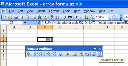
Figure 1
This brings up the Evaluate Formula dialog box. It shows which cell is being evaluated and the formula in the cell. As indicated in the dialog box, the underlined expression will be evaluated next. See Figure 2.
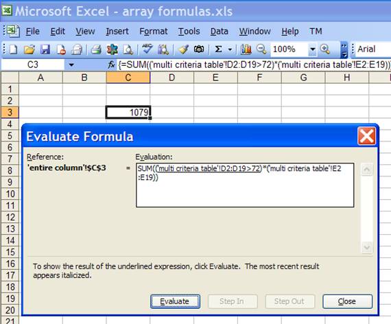
Figure 2
Click the Evaluate button to have Excel evaluate the first expression. Since this is an array formula, it generates an 18 element array of TRUE or FALSE values – the results from checking whether each cell in the range D2:D19 is greater than 72. See Figure 3.
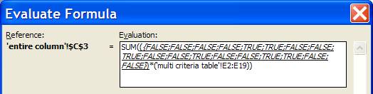
Figure 3
Click the Evaluate button to have Excel move on to the next expression (Figure 4) and click it again to have Excel include the values in the cells E2:E19 as an array (Figure 5).
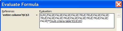
Figure 4
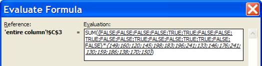
Figure 5
The next click of the Evaluate button will cause Excel to multiply each element of the first array (the 18 TRUE or FALSE values) with the corresponding element of the 2nd array. Since multiplication requires two numbers, Excel will “coerce” the Booleans into numbers using the rule that a FALSE is the same as zero and a TRUE the same as a 1. Once it does that it can then multiply the two 18 element arrays element-by-element to produce a single 18 element array as in Figure 6.
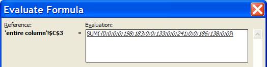
Figure 6
The final step is to carry out the SUM function and the next click of the Evaluate function does just that as in Figure 7. Once done, click the Close button to exit the Evaluate Formula dialog box.
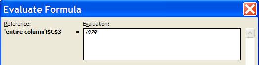
Figure 7
In reading the rest of this chapter remember one can always use the Evaluate Formula capability to figure out how Excel evaluates – or will evaluate – a particular formula.
The simplest kind of an array formula is the kind needed to deal with a function that returns a range of different results. For example, the LINEST function returns the regression coefficients of multiple variables and optionally includes a host of other statistical data. The only way to see all these results is to use LINEST as an array formula.
This form of an array formula is something I have not seen outside of my own use. Consider a list of numbers in some column (say in cells H3:H31). We want to perform the same calculation on all those numbers, say increase them by a percentage value given in I1. One way to do this is to enter, in I3, the formula =H3*(1+$I$1) and copy I3 all the way down to I31. But, this leaves the design vulnerable to a potential error. Someone might change the formula in I3 or any of the other cells in I3:I31 but not duplicate the change in the other cells. Or someone might insert a row…or delete a row…or…you get the idea.
A way to enforce consistency is to select I3:I31 and enter the array formula =H3:H31*(1+$I$1). The way Excel interprets this formula is contextual to each cell in which it is evaluated. In the context of I3, Excel interprets it as H3*(1+$I$1). In the context of I4, it interprets it as H4*(1+$I$1). Hence, functionally, it achieves the desired goal.
The advantage of this array formula is that Excel doesn’t allow one to edit a single cell that is part of an array formula. One must edit all cells at the same time! Consequently, none of the maintenance errors identified earlier in this section are possible. A positive side effect is that Excel operates on all the cells as a single “chunk” whereas in the case of 29 non-array formulas, Excel calculates each individually.
This type of an array formula is a twist on the previous type. Imagine one wants to generate a hundred random numbers between a lower value specified in B1 and an upper value specified in B2. The numbers are to go in B4:B103. One way to do this is to enter the formula =INT(RAND()*($B$2-$B$1+1)+$B$1) in B4 and copy the formula all the way to B103. This will result in 100 calls to the RAND() function whenever Excel recalculates the worksheet and the design remains vulnerable to the kind of issues discussed in the previous section.
It turns out that both INT() and RAND() are what are called “array aware” functions. If RAND is entered in multiple cells as an array formula, it returns an array of numbers equal to the number of cells it is entered into! Effectively, if we select B4:B103 and array enter the exact same formula as in the single cell case, we get 100 random numbers with a single call to RAND! And, we get all the design benefits discussed in the previous section.
In the sections above, we have seen some built-in Excel functions that are array-friendly. However, that is not true for all functions. For some that capability is meaningless by design since they always operate on arrays to return a scalar, i.e., a single result. Falling into this category are several statistics functions such as MAX, MIN, COUNT, and SUM. In other instances, the functions were just poorly designed. The most glaring array-ignorant of Excel functions is the CONCATENATE function. Given a cell range such as I3:I10, it uses I3 and ignores the rest. The array-ignorance of CONCATENATE has left a glaring hole in Excel’s string manipulation capabilities.[1] While there is a list of array-aware functions somewhere in the Microsoft Knowledge Base, it is best for one to ensure a function is array aware.
One of the criticisms of user defined functions written in VBA is that typically they are slower than an Excel formula, even a very complex array formula. While that sweeping generalization is questionable in itself, a properly designed array-aware UDF can be, to use a cliché, faster than greased lightning.[2] An example is at http://www.tushar-mehta.com/excel/newsgroups/rand_selection/vba.html#from_worksheet The function takes values entered in a range of cells and returns a list of random selections. The numbers of values returned depends on the number of cells in which the function is array-entered.
There are many functions that are documented as having arguments that take a single value. Typically, such a function also returns a single value. One example that comes to mind is the MATCH function. The first argument, the lookup-value is documented as being a single value. Further, the function returns a single value. However, some of these functions (including MATCH), will correctly handle an array of values in place of the documented single value argument. Given a range of lookup values, MATCH returns a similar sized array of values, each return value corresponding to each input value. An example should help. Consider a list of values in A8:A10. We want to check which of these values are also present in a list in B8:B10. The results are to appear in D8:D10. One way of doing this is to enter, in D8, the formula =MATCH(A8,$B$8:$B$10,0) and copy it down to D9:D10. The array alternative is to select D8:D10 and array enter the formula =MATCH(A8:A10,B8:B10,0). Note that the lookup-value (the first argument) is now a multi-cell range. See Figure 8.
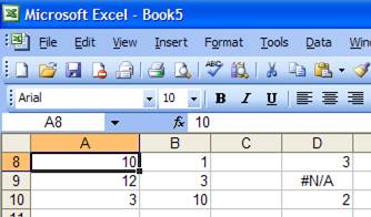
Figure 8
Another instance where this is very useful is using a range (or, interchangeably, an array) for the appropriate rows or columns argument of the OFFSET function. For example, given a list of numbers in column I starting with I3, one can extract the 1st, 4th, and 7th numbers with the formula =N(OFFSET(I3,{0;3;6},0,1,1)).[3]
One can also replace the literal array in the above formula with one that is generated by the array formula itself. This would be an example of combining two different types of array formulas and we will see an example later in this chapter and is very useful in creating a “closed” graph such as shown in xx. Such a combination of different types of array formulas plays a pivotal role in creating a custom radar (also called a spider) chart as shown in yyy.
This form of an array formula is most often used to carry out some statistical evaluation of a subset of data organized in a tabular form as shown in Figure 2 where the subset is generated based on a criterion involving more than a single column. It is even more useful when combined with a named formula that identifies a variable-sized range. Of course, a SQL query (easily generated through the use of MS Query via Data | Import External Data > New Database Query… ) will provide the same result and, actually, more that is not even possible with native Excel formulas.
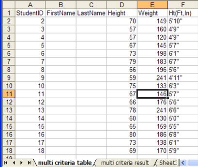
Figure 9 – a table containing information about student heights and weights
For the data above, imagine we want to know the number of students who are no taller than five feet (i.e., height<=60 inches) and who weigh at least 150 lb (weight >=150). While Excel supports database functions (see DSUM, DCOUNT, DAVG, etc. in Excel help), those functions allow only a single column in the criterion.
Before we build the appropriate array formula to give us the result it might help to review how Excel evaluates an array formula – something we did in the first section of this chapter. With the review out of the way, here’s the plan. First, we want an array of TRUE/FALSE values indicating which rows match the height criterion, with a TRUE value representing a height of 60 inches or less. Second, we want another array of TRUE/FALSE values indicating which rows match the weight criterion with a TRUE value representing a weight >= 150 lbs. Then, we multiply these two arrays element by element to get a list of 1s and 0s where a 1 represents a row meeting both criteria. Finally, we add all the elements in this last array to get a count of the rows that meet both criteria.
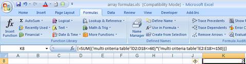
=SUM(('multi criteria table'!D2:D18<=60)*('multi criteria table'!E2:E18>=150))
This formula provides the desired result but it is not necessarily the best way to build an Excel worksheet since it suffers from three basic problems – it is poorly documented, it is not robust, and it is not easy to maintain. What do the individual components refer to? What’s D2:D18? What’s the significance of 60? Of 150?
Suppose we want to change one or both of the criteria. We would have to look up each formula in the worksheet to see if it contained a 60 or a 150 and change the value. That makes it less than easy to maintain.
But, it’s actually worse. We couldn’t simply replace every reference to 60 with the new height criterion. We would have to verify the context in which each 60 appears. That is because the formula is not properly documented. In the section ‘Array formulas and named cells’ we will look at how named cells can be used with array formulas just as they can be with regular formulas to improve documentation and maintainability.
Finally, the formula is not robust. Suppose we add new data to the original data set so that we now have data in rows 2:19. The formula does not automatically adjust to changes in the data set. We will address this limitation in the section ‘Array formulas and dynamically sized ranges’.
In the worksheet named ‘multi criteria result’ add labels and values as shown in Figure 10.
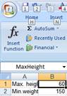
Figure 10
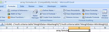
Name the cells MaxHeight and MinWeight respectively. The easiest way to name B1 MaxHeight is to click in the Name Box (at the extreme left of the formula bar), type 'multi criteria result'!MaxHeight (remember to include the single quotes) and press ENTER. Name similarly the cell B2 and on the worksheet multi criteria table the ranges D2:D18 and E2:E18.
Of course, one can just as easily use a SQL query to get the same results. And, of course, the query automatically adjusts to include additional rows as they are added to the table. Assuming the data are in a file C:\Tushar\Publishing\XL & VBA Case Studies\array formulas, the SQL syntax to get a count of the number of students would be:
SELECT Count(`'multi criteria table$'`.StudentID) AS 'Count of StudentID'
FROM `C:\Tushar\Publishing\XL & VBA Case Studies\array formulas`.`'multi criteria table$'` `'multi criteria table$'`
WHERE (`'multi criteria table$'`.Height<=?) AND (`'multi
criteria table$'`.Weight>=?)
The corresponding MS Query view would be:
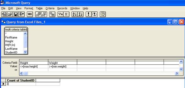
Figure 11
The additional benefit of using SQL is that one can also get the individual records in the subset, something that is much more difficult with native Excel formulas. The necessary SQL and the associated MS Query view are shown below.
SELECT `'multi criteria table$'`.StudentID, `'multi criteria table$'`.FirstName, `'multi criteria table$'`.LastName, `'multi criteria table$'`.Height, `'multi criteria table$'`.Weight, `'multi criteria table$'`.`Ht(Ft,In)`
FROM `C:\Tushar\Publishing\XL & VBA Case Studies\array formulas`.`'multi criteria table$'` `'multi criteria table$'`
WHERE (`'multi criteria table$'`.Height<=?) AND (`'multi criteria table$'`.Weight>=?)
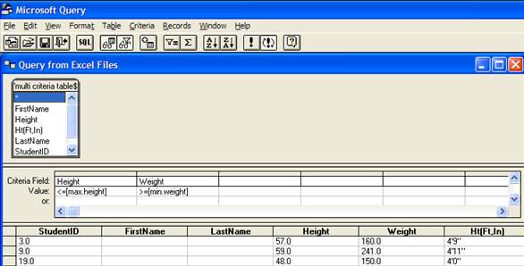
Figure 12
This is probably one of the more common uses of an array formula. While it can play a beneficial role in developing a solution, the benefits are not as significant as the extensive use of the formula might lead one to believe! As I argue in “The Case for Simplicity,” the routine use of an array formula simply to save space (like one needs to save space when an Excel workbook can have an unlimited number of worksheets each of which contains about 16.8 million cells!) is usually unwarranted. The costs from both the developer’s perspective as well as the business perspective clearly outweigh the alleged benefits. Nonetheless, since there are benefits and since this form of an array formula is extensively used, we should look at it in more detail.
The careful reader may have noticed something in the previous section that seemingly contradicts the earlier part of this chapter. In the introduction, I noted that an array formula cannot operate on an entire column (or row). Yet, in the previous section, we had an array formula that included a reference to an entire column (column A).
=SUM((OFFSET('multi criteria table'!A1,0,3,COUNTA('multi criteria table'!A:A),1)<='multi criteria result'!B1)*(OFFSET('multi criteria table'!A1,0,4,COUNTA('multi criteria table'!A:A),1)>='multi criteria result'!B2))
The key to understanding the above is to note that the function that references the entire column is not array-evaluated. The COUNTA function as used, i.e., COUNTA('multi criteria table'!A:A) is evaluated in a non-array mode. The fact that it is included inside an array formula doesn’t change that.
Create a list (an array) of the numbers 1,2,...,n
Use
=ROW(INDIRECT("1:n")), or
=ROW(OFFSET($A$1, 0, 0, n, 1))
Sort a range of numbers in descending order
Alternative 1:Use =LARGE(aRng,ROW(INDIRECT("1:"&ROWS(aRng))))
Explanation:
Alternative 2:
Use =LARGE(aRng,ROW(aRng)-ROW(OFFSET(aRng,0,0,1,1))+1)
|
Create a matrix with ones on the cross-diagonal (cells in a NxN matrix where the row number + the column number equals n+1). Used to reverse the row order or the column order of any MxN matrix. |
Harlan Grove's post on the method |
|
Reverse the elements in a column list using the INDEX function |
|
|
Reverse cells across rows and columns using the OFFSET function. |
|
|
Multiple ways to reverse the elements in a column list. |
|
|
A general formula to reverse the row order or the column order using matrix multiplication. |
[1] Laurent Longre provides a host of very useful functions, including MCONCAT, in his MoreFunc utility available at http://xcell05.free.fr/
[2] One of the more time consuming steps in the execution of a UDF is the movement of data between Excel and VBA. An array-aware function minimizes this movement both from Excel to VBA and back.
[3] The OFFSET function, when used with an array as the 2nd or 3rd argument, returns an undocumented data structure that is understood only by Excel. The N function converts the data from the internal structure into one that can be displayed or used for further analysis. Laurent Longre deserves the credit for discovering this capability of the N function.