With Excel 2007, Microsoft made several changes to the Excel 2003 feature called a List. Among the changes was renaming the feature to a Table. In this tip we look at how to create alternating color bands in a table. We also look at how we can do something similar with Excel 2003 together with some of the restrictions when it comes to the 2003 List.
When looking at a long list of items, it is always easier on the human eye to use color bands to distinguish between different rows. Excel does this by default when one creates a table in Excel.
Create a table in Excel 2007 use Insert | Tables
group | Table button. The default result is bands of alternating shades of blue.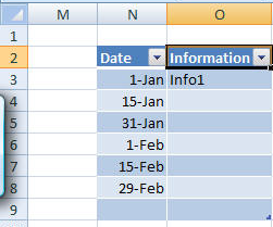
The Excel 2003 version is called a List and created with Data | List >
Create List... However, there is no default banding. 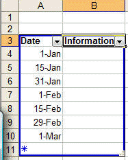
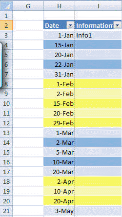
While the default Excel 2007 banding is helpful, it is not content-sensitive. In the above example, with the data in chronological order, it would help if we could band the data by month - as I do with the transactions for my checking account.
Of course, even that may not be enough. If there is a long list of items for a single month, it would help to use a different color for adjacent months and then shades of that color within the month thereby creating bands within bands.
We will use conditional formatting (c.f.) in both Excel 2007 and Excel 2003 to create the bands.
The typical and arguably "straight-forward" way to use conditional formatting is to embed the formula that lets us differentiate between the months in the c.f. condition. After a brief discussion on some serious limitations about this approach, we will explore a more transparent way of creating the bands. Finally, we will wrap up the Excel 2007 section by looking at how to create the bands within bands
To start, select the table then select the Home tab | Styles group | Conditional Formatting drop-down | Manage Rule... button.
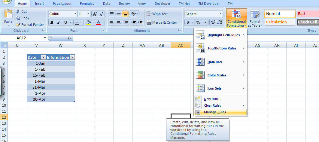
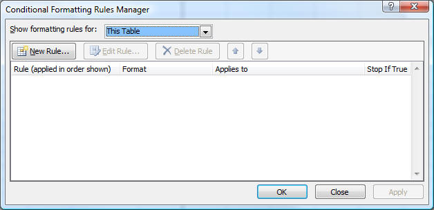
This brings up the new (new to Excel 2007, that is) C.F. dialog box. Note how the 'Show formatting rules for' drop down refers to 'This Table.' This is important since we want the conditional formatting to automatically apply to new rows as we add them.
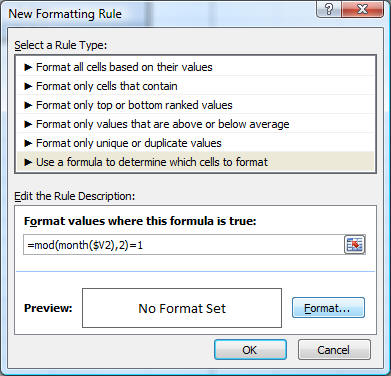
Click the 'New Rule...' button and in the resulting dialog box select 'Use a formula to determine which cells to format.' Then, enter the formula as shown. Note that V2 refers to the header of the Date column in the table.
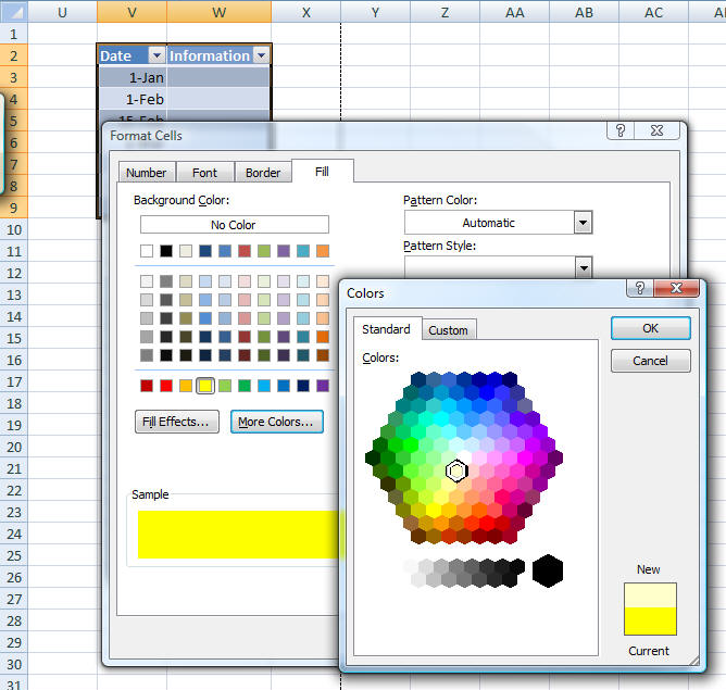
Next, click on the Format... button and select an appropriate color from the Fill tab. If necessary, click the More Colors... button and select an appropriate color. Note that this level of control over the color is available only in Excel 2007.
The final C.F. should look as below. The formula checks if the month (expressed as a number) is an odd number (January, March, May, etc. will be 'odd' months). If so, the table row fill will be the specified color.
Do the same for months with even numbers (February, April, June, etc.) The formula is slightly different and the Fill color is, of course, another color.
The Manage Rules... dialog box should now look as below.
The result of the above c.f. rules is shown below.
Bands in Excel 2003