Gregory L on Feb. 17, 2013
very straight forward examples. Good step by step presentation.
This requires a two step process. The second step we have already seen since it is exactly the same as the parameterized query discussed in Query 4. What is new is the source for the parameter. Since it must be a zip code already in the database, the only way we can know what zip codes to consider is with a database query. The selection drop down box will come from use of Excel's Data Validation capability.
First, create a query to get the list of valid zip codes. This is pretty straightforward with just one twist. The typical query we have used so far returns one row per database record. That would mean we would get list of zip codes that include all sorts of duplicate entries. We need to restrict the returned result to one row per unique zip code. It's quite easily specified through a query property.
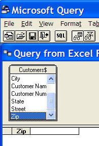
Once again, given that we know how to link to MS Query, how to add tables to a query within MS Query, how to add fields to the query, and how to return data to Excel, we can expedite building this query. Once in MS Query add the Customers table to the query and add the Zip field to the selected fields pane.
Then, use View | Query Properties... and check the option Unique Values Only
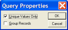
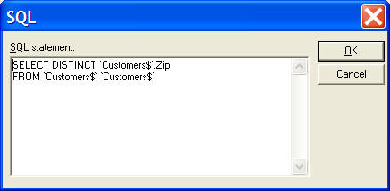
What this does is to eliminate duplicate rows. The associated SQL, for those interested, contains the DISTINCT clause.
Back in Excel, put the result in some cell. I picked B4.
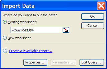
The result will look like:
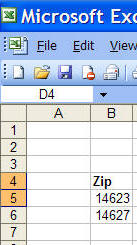
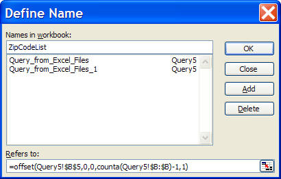
Next, add a named formula (Insert | Name > Define...) identifying the range containing the returned zip codes. Now, ZipCodeList refers to as many zip codes entries as are returned by MS Query.
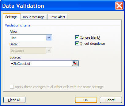
Next, we add a data validation condition to some cell, say D5. Select D5 then Data | Validation... In the resulting dialog box use the Allow drop-down to pick List and in the Source field enter the name of the formula from above.
From here on end the rest of the design is identical to that of Query 4 except that the parameter source will be D5 rather than B4. The result should look like:
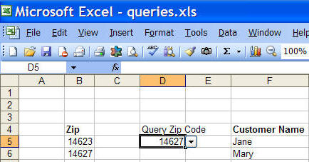
Of course, for aesthetic appeal, one might want to hide column B and add an appealing title to the worksheet.